|
Lecture Notes
I. Defining Cost Types
A.
Introduction
1. The last two chapters were an in-depth
exploration of demand.
2. This chapter will explore costs, the key
determinate of supply.
B. Costs
are the dollars paid for the factors of production.
1. Explicit
costs require an out-of-pocket expenditure, e.g., wages,
materials, and overhead.
2.
Implicit costs do not require an outlay, e.g.,
forgone interest on
invested capital, forgone rent a company could receive by renting
a facility used
in the business,
forgone wages for uncompensated
efforts by family members
in a family-operated business, forgone
entrepreneurial income you
could earn by
managing another
business. Included a normal return on investment, which is the
minimum
amount required to keep resources employed at their
current use.
3.
Opportunity Costs_
C.
Short run versus
long run costs
1. In the short
run costs are both fixed and variable.
a.
Fixed costs do not vary with production, e.g.,
plant and
equipment,
property taxes, most overhead, etc.
b.
Variable costs vary directly with
production, e.g., labor and
materials
c.
Marginal cost is the change in total costs
which results from
making
one more unit.
2. In the long
run all costs are variable as fixed costs may increase.
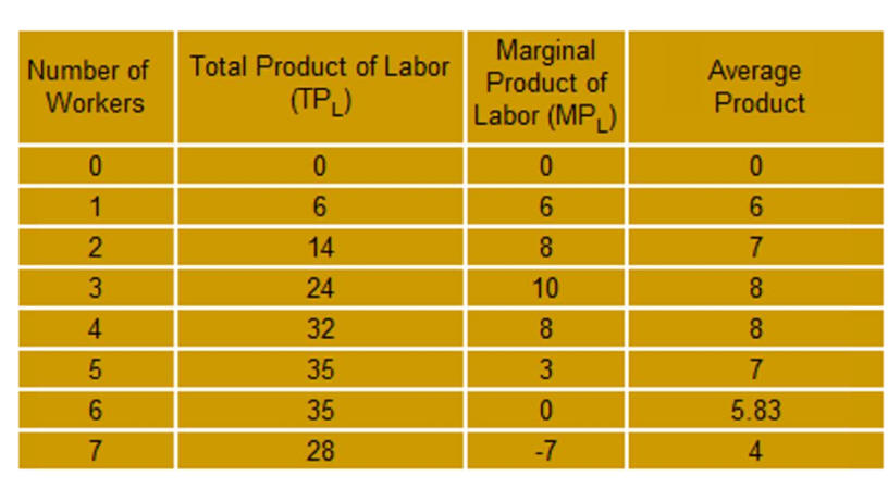
D. Diminishing returns:
1. Adding
a variable resource (labor) to a fixed resource (capital) will
increase production for a while.
2. At some point the rate
of increase declines-turns negative.
3. Diminishing returns affects labor
cost and cost of production.
4. Example: When eating at my
mother's house I would say
using three people to do the dishes didn't make sense
because
the
third person just got in the way. She agreed so me and
my sisters did the
dishes.
5.
Diminishing returns - Wikipedia
has additional information.
6.
Econ in 60 Seconds
Law of Diminishing Marginal Returns
reviews
diminishing returns and previews section III on labor
productivity.
E.
Accounting profits
versus economic profits
1. Accounting
profit is revenue minus explicit costs.
2. Economic
profit is revenue minus explicit plus implicit costs.
3. Since
implicit cost includes a payment for the risk factor part of
interest and payment for entrepreneurial skill.
4. This means
a.
Normal Profit is a cost to economists and paid for
as an
explicit cost.
b. In the
long run competition causes economic profit to be zero.
F. Related topics
1.
Ignore Sunk Costs
29 min audio
2.
Introduction to Managerial Accounting 8 min. video
3.
Managerial Accounting Internet Library
4. Accounting
for Managers has free books
5.
Econometrics
video lectures
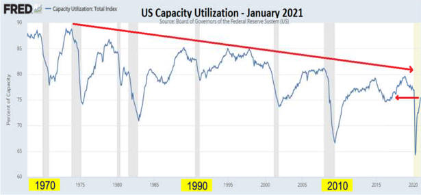
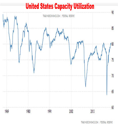
US Capacity Utilization Back to 2016 Levels - The Sounding Line
|
Supplemental
Political Economy
Stuff
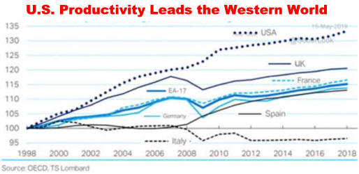
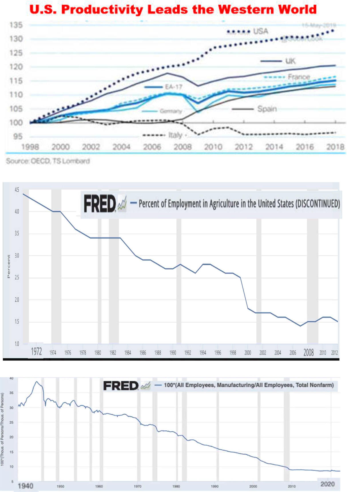
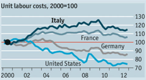
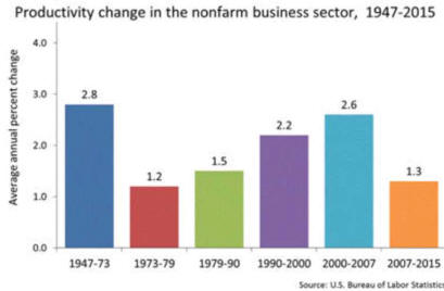
Current Slow Down is Not Unprecedented
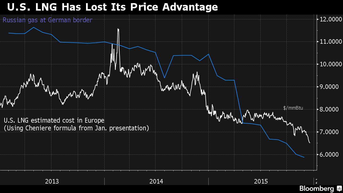
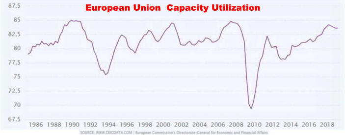
With Asian Competition,
Some Manufacturing Became Less Profitable
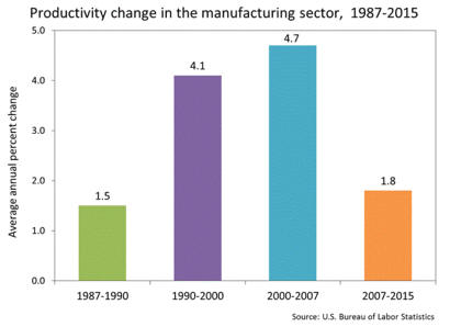
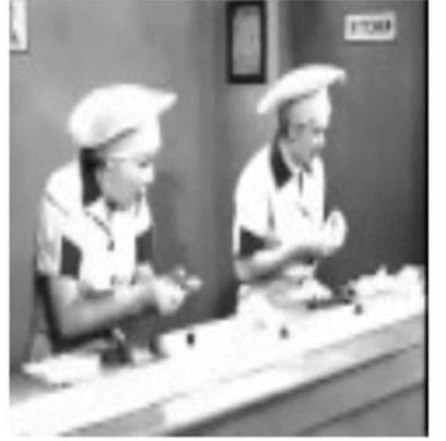
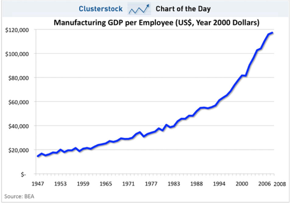
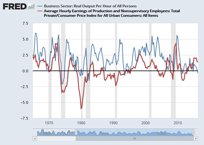
Service Productivity Improved
Because Fewer Workers Needed
|